packages = c('tidyverse','knitr', 'scales','sf', 'tmap', 'highcharter', 'plotly','ggstatsplot','lubridate','ggridges','ggrepel')

for(p in packages){
  if(!require(p, character.only = T)){
    install.packages(p)
  }
  library(p, character.only = T)
}Take-home Exercise 3
The Task
In this exercise, we are required to uncover the salient patterns of the resale prices of public housing property by residential towns and estates in Singapore.
1. Introduction
As of 2020, 78.7% of Singaporeans live in public housing. There are three forms of housing in Singapore: lessee-occupied public housing, resale public housing, and rental public housing.
In Singapore, the majority of public housing is under lessee-occupied. Under Singapore’s home leasehold ownership scheme, dwelling units are given on a 99-year leasehold basis to applicants who meet certain income, citizenship, and property leasehold ownership conditions. New lessee-occupied flats will be sold via the Build-To-Order and Sale of Balance Flats programs. Lessee-occupied public housing, on the other hand, can be sold in a resale market, subject to certain regulations. The government has no control over resale market prices. Therefore, this exercise aims to examine the distribution and prices of public housing in Singapore, which may be useful in assisting readers in making informed decisions when analyzing the resale market.
2. Data
We will be using “Resale flat princes based on registration date from Jan-2017 onwards” which is available at Data.gov.sg. For this exercise, we will only be looking at 2022 data and focusing on 3-Room, 4-Room and 5-Room types.
3. Data Preparation
Ensure following packages are installed.
First, we use the read_csv() function of the readr package to import Resale flat princes based on registration date from Jan-2017 onwards csv dataset into the R environment.
SGResale_2022 <- read_csv("data/resale-flat-prices-based-on-registration-date-from-jan-2017-onwards.csv")read.csv() function from base R has the same functionality as read csv().
Note: read csv() function is preferred over read.csv() because it preserves the whole variable name. read.csv() replaces any spaces in variable names with a period (.), where the names of the variables will be changed.
As we will only be looking at 2022 data and focusing on 3-Room, 4-Room and 5-Room types, we perform the following filters on the dataset.
Filter dataset where flat_type is 3-Room, 4-Room & 5-Room
Filter dataset based on Year 2022
SGResale_2022 <- subset(SGResale_2022, flat_type == "3 ROOM" | flat_type == "4 ROOM" |flat_type == "5 ROOM")
SGResale_2022$Year = substr(SGResale_2022$month, 1, 4)
SGResale_2022 <- subset(SGResale_2022, Year == "2022")
4. Visualization
4.1 Time Analysis
By plotting both resale volume and resale price over time, we can see how the HDB prices varies across Year 2022.
We group the dataset by month and aggregate by average price:
SGResale_2022_bymonth <- SGResale_2022 %>%
  group_by(month) %>%
  mutate(average_price = mean(resale_price))
Plotting both axis on the same graph:
 ggplot(data = SGResale_2022_bymonth) +
  # Plot the price
  geom_bar(mapping = aes(x=month), fill="khaki2") +
  # Change position of price
  geom_point(mapping = aes(x=month, y=average_price/300), color = "royalblue4") +
  geom_line(mapping = aes(x=month, y=average_price/300), group = 1, color = "royalblue4") +
  # Add a second Y axis
  scale_y_continuous(sec.axis = sec_axis(~.*300, name = "Resale price (SGD)", labels = comma)) +

  # Change color of the second Y axis to match with the color of resale price
  theme_minimal() +
  theme(axis.ticks.y.right = element_line(color = "royalblue4"),
        axis.text.y.right = element_text(color = "royalblue4"),
        axis.title.y.right = element_text(color = "royalblue4")) +

  # Adjust styles, lables and add title
  theme(axis.text.x=element_text(angle = 35)) +
  labs(title = "HDB resale market in Year 2022", y="Resale volume",
       x = "Month", caption = "Source of data: Singapore Housing and Development Board")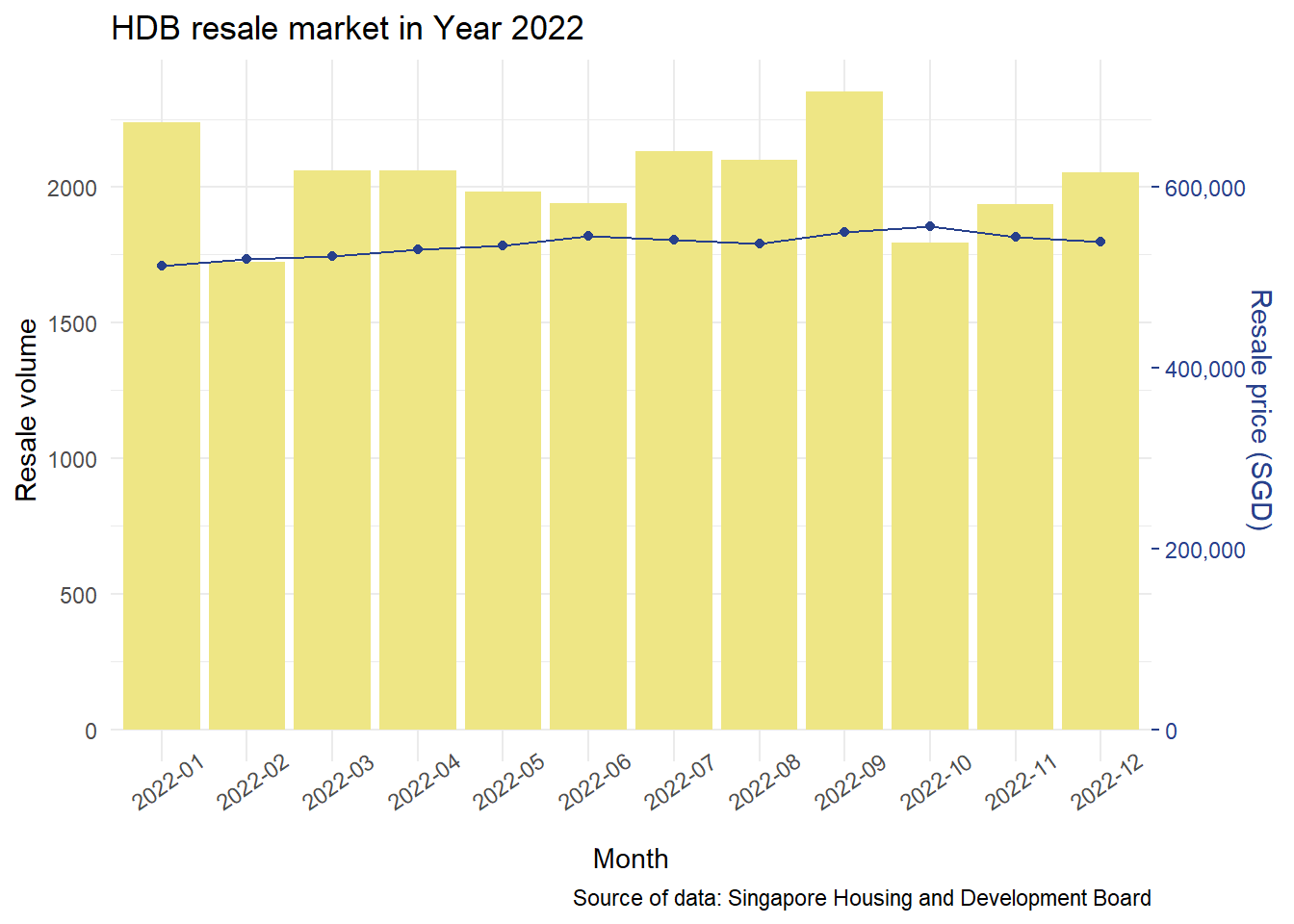
We observe that the overall resale price for HDB resale market is around the same throughout 2022. However, there was a huge spike in Sept and dropped further in Oct. This may be due to the cooling measure announced by the government which took immediate effect on 30 September 2022.
4.2 Flat Type Analysis
Next, we plot boxplot by quarter and across flat type to see how prices fluctuated in the last year for different flat types.
SGResale_2022_byflat <- SGResale_2022 %>%
  group_by(flat_type) %>%
  mutate(quarter = quarter(ym(month)),
price_per_sqm = resale_price/floor_area_sqm)ggbetweenstats(
data = SGResale_2022_byflat,
x = flat_type,
y = price_per_sqm,
type = "np",
plot.type = "boxviolin",
title = "HDB resale prices in 2022 by flat type",
xlab = "Flat type",
ylab ="Price per sqm (SGD)")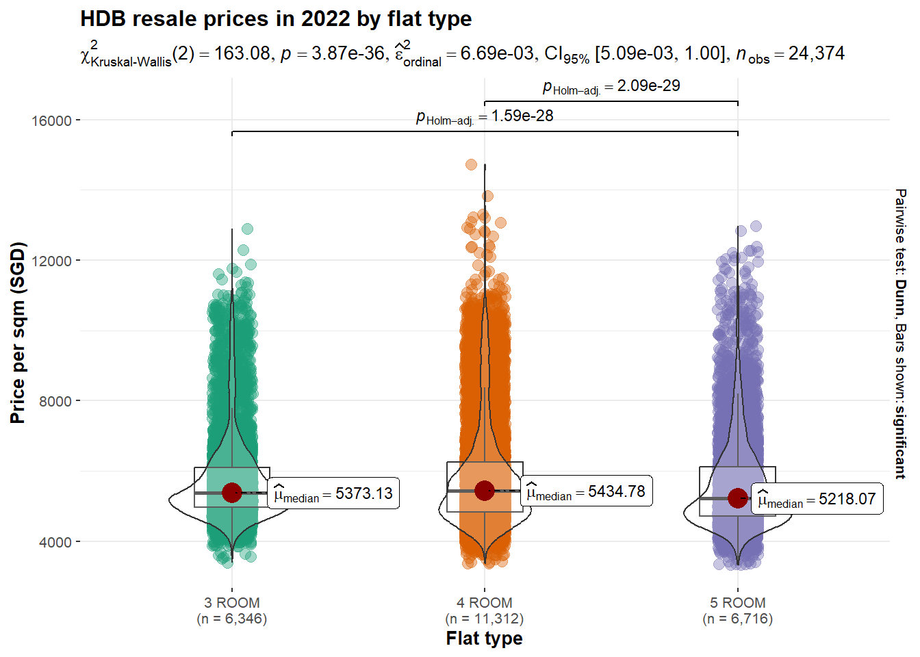
The overall p-value of the ANOVA test between Type of Flat and Resale Price per sqm is 0.00 < 0.05, which suggests that we can reject the null hypotheses. This means that each flat type has a different mean resale price.
ggplot(data = SGResale_2022_byflat, mapping = aes(x = flat_type, y = price_per_sqm)) +
   geom_boxplot(color = "black") +
  theme_minimal() +
  theme(legend.position = "top") +
  scale_fill_viridis_d(option = "A") +
  # Adjust lables and add title
  labs(title = "HDB resale prices in 2022 by flat type", y="Price per square metre (SGD)",
       x = "Flat type", caption = "Source of data: Singapore Housing and Development Board")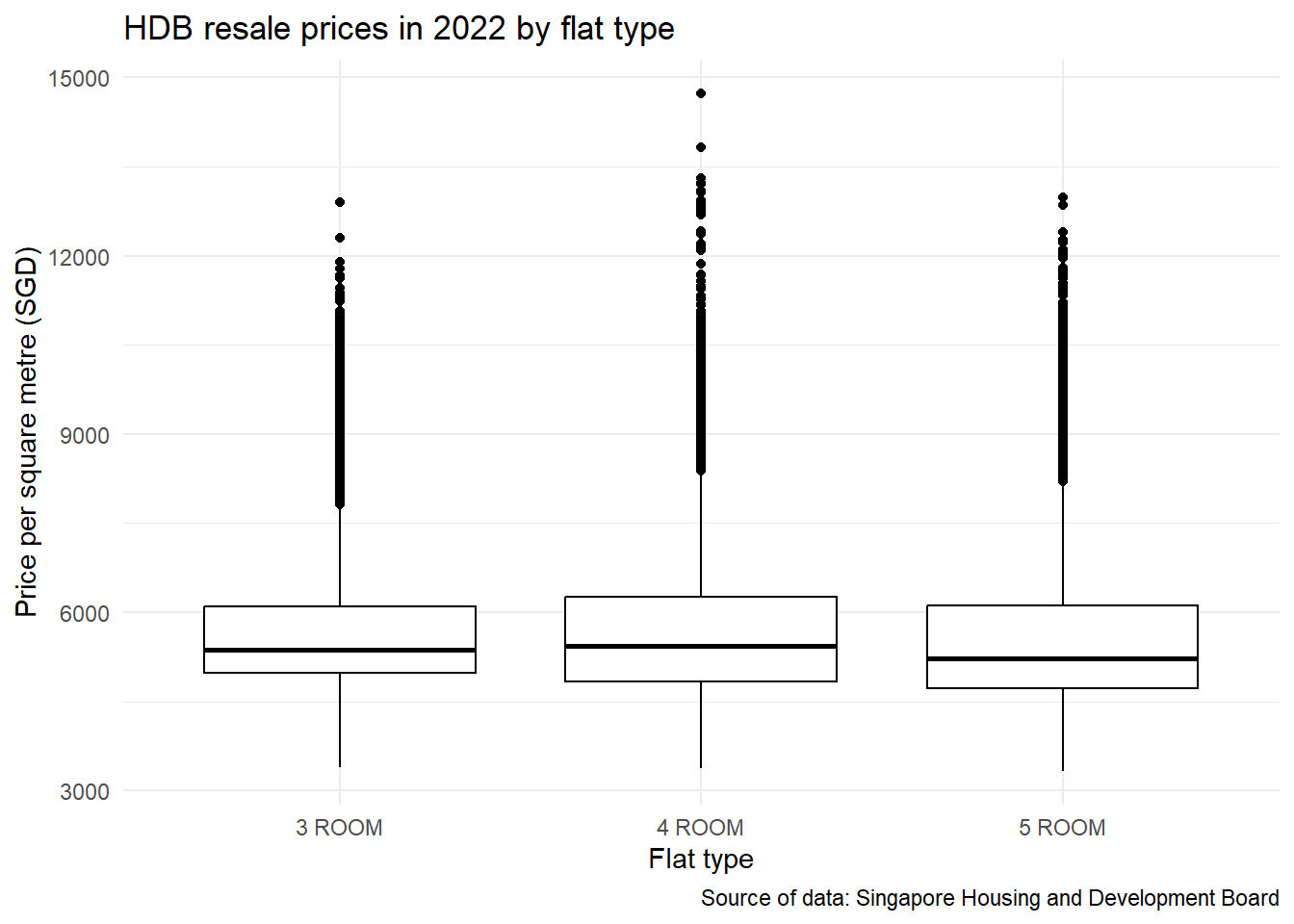
We observe that the price per square metre for 5 Room is the lowest. Interestingly, 4 Room and 3 Room price per square metre are comparable with 4 Room slightly higher. However, this could be due to many outliers with extremely high prices per square metre in 4 Room.
To analyze further into time, we use lubridate package to transform month into quarters.
ggplot(data = SGResale_2022_byflat, mapping = aes(x = flat_type, y = price_per_sqm)) +
  # Make grouped boxplot
  geom_boxplot(aes(fill = as.factor(quarter)), color = "gray") +
  theme_minimal() +
  theme(legend.position = "top") +
  scale_fill_viridis_d(option = "D") +
  # Adjust lables and add title
  labs(title = "HDB resale prices in 2022 by flat type", y="Price per square metre (SGD)", fill = "Quarter",
       x = "Flat type", caption = "Source of data: Singapore Housing and Development Board ")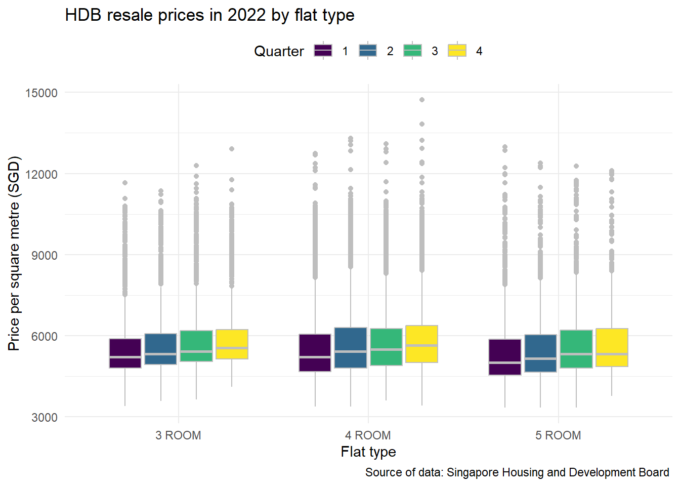
Here we observe that in all flat types, the average price per square metre increases from Q1 to Q4.
4.3 Geographical Analysis
Next, we will group the dataset by town to find if the geographical effects of the flat’s location on its resale price.
SGResale_2022_psqm <- SGResale_2022 %>%
  mutate(price_per_sqm = resale_price/floor_area_sqm)
We plot the the distribution of price per square metre using rigdeline plot using ggridges package.
We observe that Central area has the highest price but the distribution is scattered. There is a diverse range of housing in the central area, including skyrise apartments and older homes which could be contributing to this distribution. There are two crests in city fringe neighborhoods such as Queenstown and Kallang/Whampoa, which may indicate that the neighborhood is diverse and contains both costly and inexpensive houses. Observing neighborhoods like Choa Chu Kang, Woodlands, and Sembawang with high concentrations of prices at each crest, it is evident that these are predominantly residential neighborhoods. Considering this, we can conclude that residential housing with mixed housing concentration improves affordability.
SGResale_2022_bytown <- SGResale_2022_psqm %>% group_by(town)

  # Plot the neighborhoods in an ascending order of price per sqm
  ggplot(data = SGResale_2022_bytown, mapping = aes(x = price_per_sqm, y = reorder(as.factor(town),-price_per_sqm),
                       fill = after_stat(x)
                       )) +
  geom_density_ridges_gradient(color = "white") +
  scale_fill_viridis_c(option = "C") +
  theme_minimal() +

  # Remove legend, grid line add title
  theme(legend.position = "none") +
  theme(panel.grid = element_blank()) +
  labs(title = "HDB resale prices in 2022 by neighborhood", x = "Price per square metre (SGD)", y = "",
       subtitle = "Neighborhood exhibit large differences",
       caption = "Data: Housing and Development Board, Singapore")
Picking joint bandwidth of 247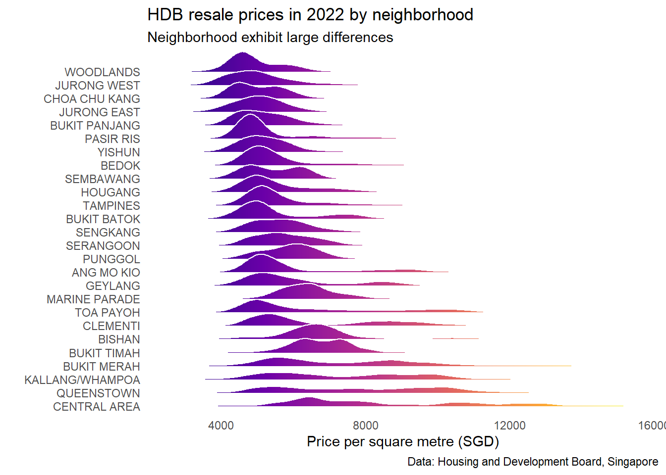
We drill further into each neighborhood by flat types to see if location had a great effect on flat resale prices. Generally, central area had the most expensive flats by mean price per square meter, followed by Queenstown and Kallang/Whampoa in 2022. This was also observed in 4 Room & 5 Room, the reason could be that these location are in close proximity to the city centre, hence are more expensive especially for those who value connectivity and easy access to the Central Business District (CBD).
However, when we look at 3 Room, surprisingly Pasir Ris was significantly higher than other neighborhoods for 3 Rooms, followed by Punggol & Sengkang. A possible reason for the higher prices in Punggol and Sengkang is the HDB flats that have fulfilled their Minimum Occupation Period (MOP) in 2022 being located in these two towns.
SGResale_2022_bytown <- SGResale_2022_psqm %>% group_by(town)

ggplot(SGResale_2022_bytown, aes(x=reorder(town, price_per_sqm), y=price_per_sqm)) +
  geom_boxplot() +
  labs(title="Average Flat Resale Price (psm) by Town for all room types in 2022 ",
       x="Town",
       y="Resale Price ($ psm)") +
  theme_classic() +
  theme(plot.title = element_text(size=10, hjust=0.5),
        axis.title.x = element_text(size=10),
        axis.text.x = element_text(angle=35, hjust=1),
axis.title.y = element_text(size=10)) 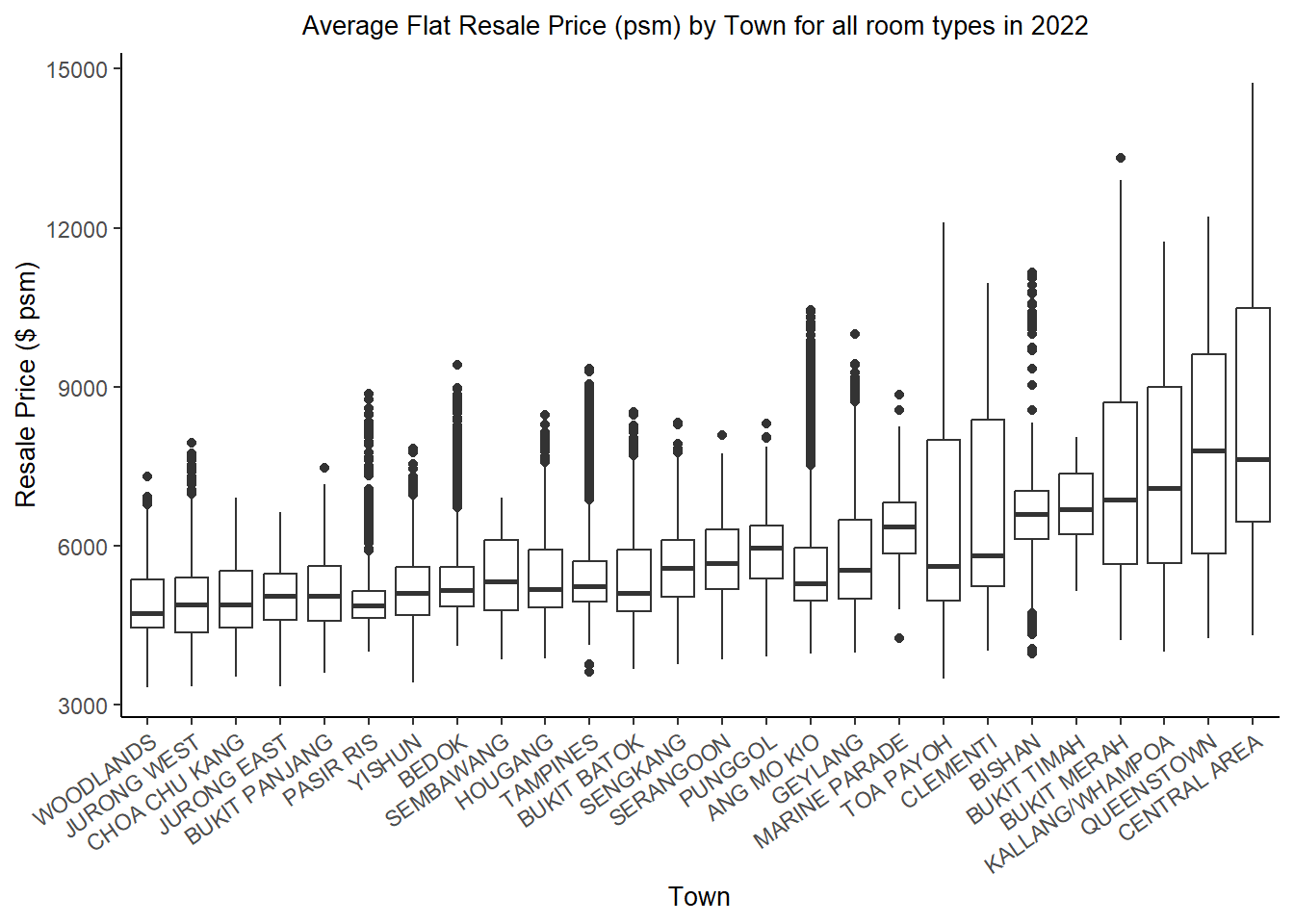
type <- "3 ROOM"
SGResale_2022_bytown <- SGResale_2022_psqm %>% group_by(town) %>% filter(flat_type==type)

ggplot(SGResale_2022_bytown, aes(x=reorder(town, price_per_sqm), y=price_per_sqm)) +
  geom_boxplot() +
  labs(title=paste("Average Flat Resale Price (psm) by Town for", str_replace(lapply(type, tolower), '_', '-'), "flats"),
       x="Town",
       y="Resale Price ($ psm)") +
  theme_classic() +
  theme(plot.title = element_text(size=10, hjust=0.5),
        axis.title.x = element_text(size=10),
        axis.text.x = element_text(angle=35, hjust=1),
axis.title.y = element_text(size=10)) 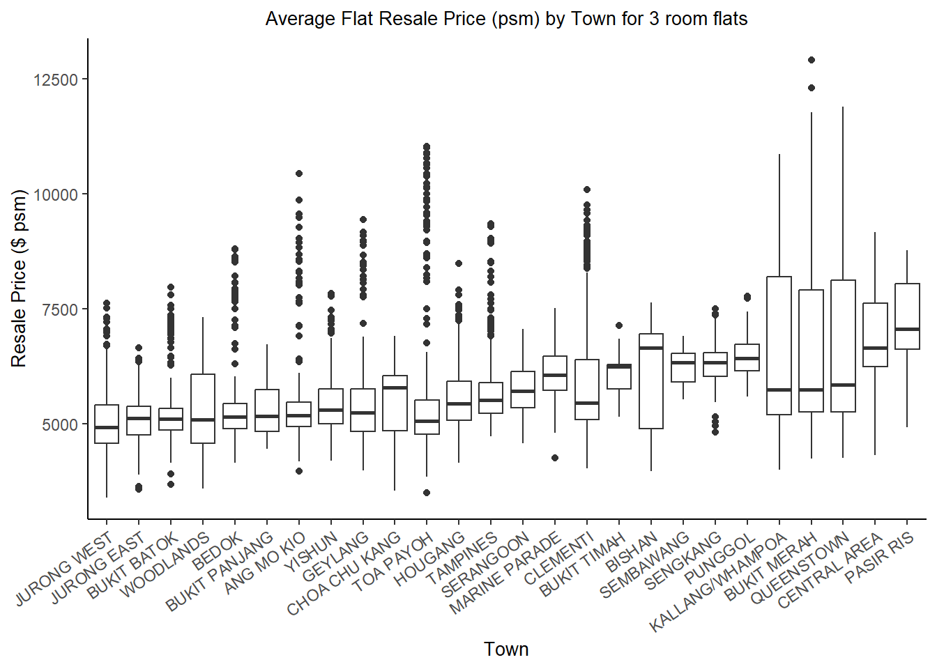
type <- "4 ROOM"
SGResale_2022_bytown <- SGResale_2022_psqm %>% group_by(town) %>% filter(flat_type==type)

ggplot(SGResale_2022_bytown, aes(x=reorder(town, price_per_sqm), y=price_per_sqm)) +
  geom_boxplot() +
  labs(title=paste("Average Flat Resale Price (psm) by Town for", str_replace(lapply(type, tolower), '_', '-'), "flats"),
       x="Town",
       y="Resale Price ($ psm)") +
  theme_classic() +
  theme(plot.title = element_text(size=10, hjust=0.5),
        axis.title.x = element_text(size=10),
        axis.text.x = element_text(angle=35, hjust=1),
axis.title.y = element_text(size=10)) 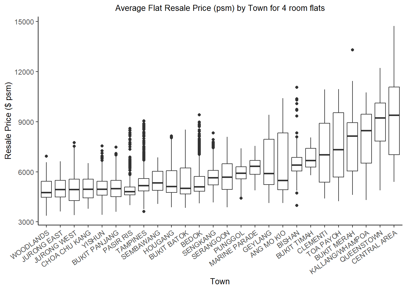
type <- "5 ROOM"
SGResale_2022_bytown <- SGResale_2022_psqm %>% group_by(town) %>% filter(flat_type==type)

ggplot(SGResale_2022_bytown, aes(x=reorder(town, price_per_sqm), y=price_per_sqm)) +
  geom_boxplot() +
  labs(title=paste("Average Flat Resale Price (psm) by Town for", str_replace(lapply(type, tolower), '_', '-'), "flats"),
       x="Town",
       y="Resale Price ($ psm)") +
  theme_classic() +
  theme(plot.title = element_text(size=10, hjust=0.5),
        axis.title.x = element_text(size=10),
        axis.text.x = element_text(angle=35, hjust=1),
axis.title.y = element_text(size=10)) 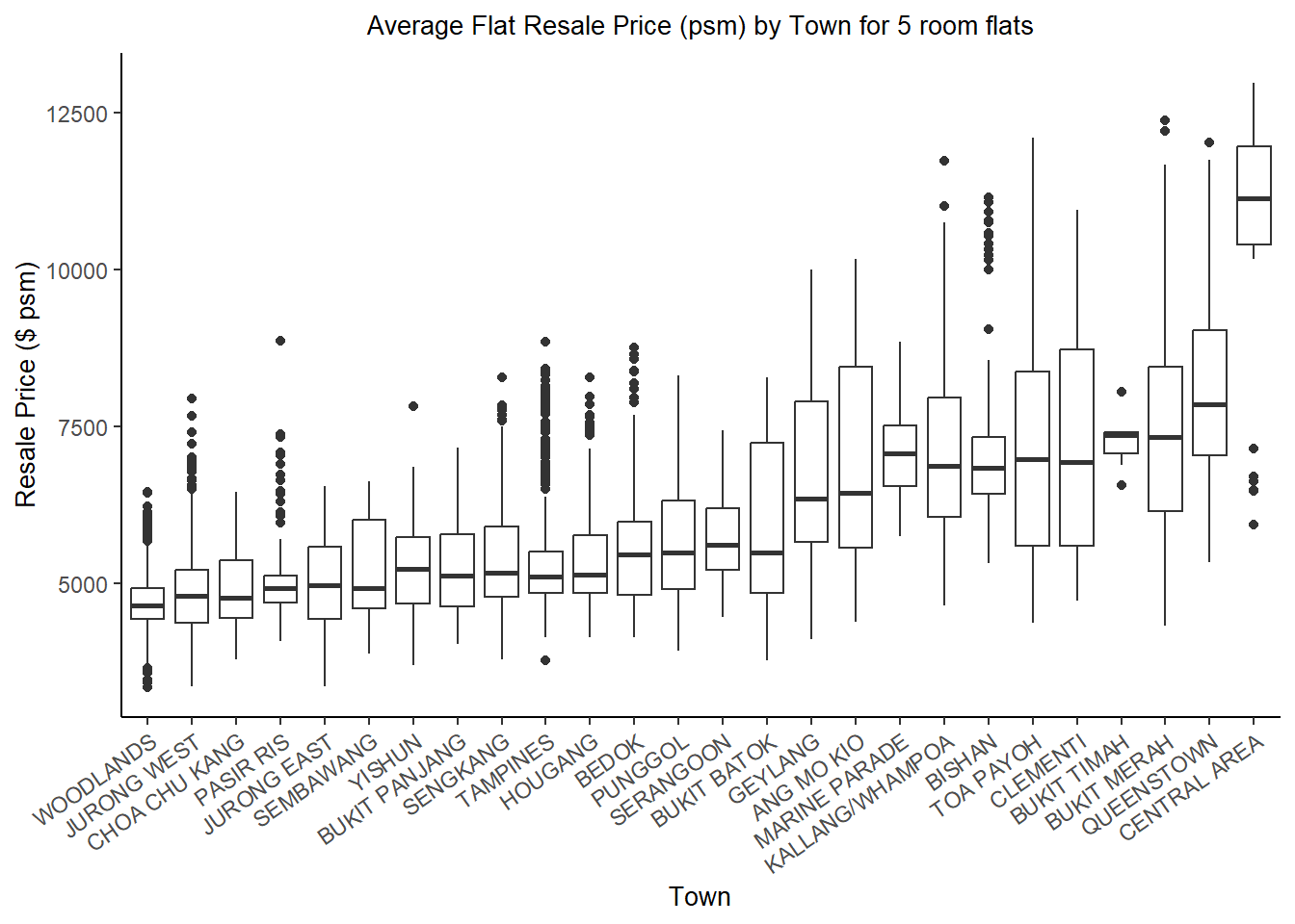
Overall, we observe that the location and type of HDB flat greatly influences the resale price of the property. This is likely because HDB flats in certain parts of the city are more sought-after due to their proximity to amenities and other factors, while certain types of flats may be more desirable due to their size or layout. This is why prospective buyers should consider all these factors carefully before making a purchase.
5. References
Share of households in condos, apartments up almost 5 percentage points as proportion in HDB flats slips 3.7 points: census. Business times. (2021, June 19). Retrieved February 13, 2023, from https://www.businesstimes.com.sg/singapore/economy-policy/share-households-condos-apartments-almost-5-percentage-points-proportion
Koo, A. (2022, October 3). New property cooling measures in 2022 and the HDB buyers, downgraders & upgraders who could be affected by the latest changes. DollarsAndSense.sg. Retrieved February 14, 2023, from https://dollarsandsense.sg/new-property-cooling-measures-2022/
HDB resale prices Q3 2022: Singapore Estates ranked from most expensive ... (2022, October 31). Retrieved February 14, 2023, from https://www.propertyguru.com.sg/property-guides/pgf-hdb-resale-flat-estates-price-most-expensive-cheapest-55414